December 27, 2022
In this article, I describe the benefits of accelerating parallel computation workloads with GPUs using the NVIDIA CUDA API and how it can be applied to popular applications of parallel computing, such as deep learning.
Disclaimer: The concepts and project discussed in this article are a part of the course offering of ECE 408 / CS 483 at the University of Illinois Urbana-Champaign. To maintain academic integrity, the code snippets below come from external sources (which are cited) and are not my own personal work for the course nor the project.
Many applications of parallel computing, such as scientific computing, machine learning, and deep learning require a large amount of numeric computation. GPUs are particularly well-suited for these applications due to their ability to do high-throughput work, when compared to CPUs.
Modern GPU architectures support computation over thousands of threads, which are organized into blocks. Blocks are organized into grids. Within each block, threads execute instructions in groups called warps.
Fortunately, many popular computational patterns, such as vector mathematics, matrix multiplication, discrete convolution, scanning, and reduction map nicely into this three-dimensional grid-like pattern.
A very simple example of parallelizing computation is vector addition. Let’s say we have two vectors: \(a, b \in \mathbb{R}^n\). We want to compute \(c_i = a_i + b_i\). The sequential CPU code in C++ may look something like this:
// Source: https://www.olcf.ornl.gov/tutorials/cpu-vector-addition/
// Sum component wise and save result into vector c

for (int i = 0; i < n; i++) {
    c[i] = a[i] + b[i];
}
We recognize that every output element of \(c\) can be calculated independent of every other output element. We can assign one output element of \(c\) to one GPU thread. Each thread determines which element of \(c\) it computes based on its block and thread index (which block it is a part of and its position in that block). We must also be careful to avoid reading and writing out of the bounds of the input and output arrays.
// Source: https://www.olcf.ornl.gov/tutorials/cuda-vector-addition/
// CUDA kernel. Each thread takes care of one element of c

__global__ void vecAdd(double *a, double *b, double *c, int n) {
    // Get our global thread ID
    int id = blockIdx.x * blockDim.x + threadIdx.x;

    // Make sure we do not go out of bounds
    if (id < n)
        c[id] = a[id] + b[id];
}
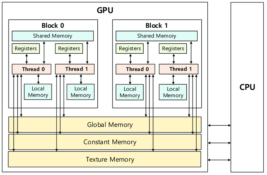
Source: Efficient Parallel Implementations of LWE-Based Post-Quantum Cryptosystems on Graphics Processing Units by SangWoo An and Seog Chung Seo is licensed under CC BY 4.0
The memory hierarchy of NVIDIA GPUs presents opportunities to optimize the efficiency of memory accesses in CUDA kernels.
Global memory is the primary memory space of the GPU. Calls
to CUDA API functions like cudaMalloc,
cudaMemset, and cudaMemcpy can be used
to interact with global memory to allocate, initialize, and
transfer data between the device (GPU) and host (CPU).
Shared memory is allocated per-block and shared among threads
of the block. A potential optimization using shared memory is to
load tiles of frequently reused data into shared memory. This
may require barrier synchronization using
__syncthreads() which reduces parallelism but is
needed to satisfy dependencies. Rather than fetching data from
global memory, which is a slow process taking many cycles,
threads can quickly read data loaded into the shared memory
tile. An example usage of this optimization is tiled, shared
memory matrix multiplication.
Constant memory is an area of memory which serves essentially as a read-only cache. Data can be copied to the device’s constant memory and similar to shared memory, accesses to constant memory run much faster than accesses to global memory. An example usage of this optimization is loading a convolution mask into constant memory.
Memory coalescing refers to an access pattern in which several threads of a warp access adjacent memory locations.
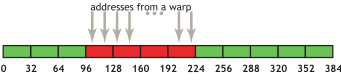
Source: NVIDIA CUDA C++ Best Practices
With coalesced accesses, we move closer to maximizing global memory bandwidth, as we make maximal use of data returned in DRAM bursts.
A convolution layer of a convoluational neural network performs an element-wise dot product between the input and mask, which “slides” across the input, to produce the output. It can be used in applications such as image processing to perform blurring, sharpening, or edge detection.
Source: 2D Convolution Animation by Michael Plotke is licensed under CC BY-SA 3.0
The parallelized convolution layer runs in a LeNet-like neural network architecture. To perform inference with a convolutional layer, we perform a parallel convolution to compute every output element for each image per batch, for all output feature maps. Images may also have several channels, for example RGB values, over which the convolution is computed.
The baseline sequential CPU code runs inference of a batch of 10,000 images in roughly 95s. The baseline parallelized GPU code runs the same batch in roughly 90ms for a 99.9% speed improvement. Further specialized optimizations reduce the runtime to roughly 69ms from the baseline parallel implementation.